Superposition, Phase Diagrams, and Regularization
I was reading through "Toy Models of Superposition" by Anthropic, which I highly recommend. The authors present the phase diagram of a small neural network, including both the theoretical and empirical versions. However, they do not apply any form of regularization in their analysis, which piqued my curiosity about the effects of superposition. As a result, I decided to experiment with this idea, and these are the results I came up with. I also aimed to explain everything in a simple way so that everyone could understand it.
Let's first introduce the neural network and the data. This will make the explanations in the following sections much simpler.
We will consider a very simple neural network: \[f(x;W) = \operatorname{ReLU}(xWW^T) \] Here, \(x\) represents the input data, while \(W\) is the network parameter—a simple matrix. A final \(\operatorname{ReLU}\) activation function is applied at the end (for those unfamiliar, \(\operatorname{ReLU}(x) = \max(x, 0)\)). Now, let's assume that the input data, \(x\), is an n-dimensional vector with entries between \(0\) and \(1\)---that is, \(x \in [0, 1]^n\). The weight matrix \(W\) belongs to \(\mathbb{R}^{n \times m}\), so \(xW\) is an m-dimensional vector, i.e., \(xW \in \mathbb{R}^m\). Finally, \(xWW^T\) is an n-dimensional vector once again, meaning \(xWW^T \in \mathbb{R}^n\).
We will train the network \(f\) using a simple reconstruction loss—the mean squared error. This means we will encode \(x\) into a feature space (typically lower dimensional) and then decode it back into the original space. Thus, our loss function will be: \[\mathcal{L}(x;W) = \frac{1}{n} \sum_{i=1}^n (f(x;W)_i - x_i)^2 \]
It should be fairly clear that our network will be optimal when \(\forall x: f(x; W) = x\), resulting in \(\mathcal{L}(x; W) = 0\). It's also evident that this occurs when \(W = I\), the identity matrix, since \(f(x; I) = \operatorname{ReLU}(xII^T) = x\). The same holds for any orthogonal matrix however, if we aim to encode \(x\) into a lower-dimensional space, where \(m < n\), the identity matrix \(I\) is no longer a valid option.
Let's simplify even further and assume \(n = 2\) and \(m = 1\). In this case, we will have only two weights to work with, and we need to encode two entries from \(x\) into a single real value. Let's refer to each entry as a feature. Ultimately, there are limited options:
- We can encode only the first feature, \(W = [1, 0]\).
- We can encode only the second feature, \(W = [0, 1]\).
- Or, we can encode a combination of both features. For example, \(W = [1, -1]\), meaning the first feature will be encoded on the positive semi-axis of the reals, while the second feature will be encoded on the negative semi-axis. In other words, the two features are superimposed.
Now, our question becomes: when does it make sense to superimpose two features rather than choosing only one? To answer this question, we will set up a very simple experiment. Firstly, we will introduce a sparsity term for the data, \(s \in [0, 1]\). Specifically, we will set each feature to \(0\) with probability \(s\). Additionally, we will introduce two importance terms, \(r_1\) and \(r_2 \in [0, 1]\), which will represent the importance of each feature. Finally, we will add a regularization term, \(\lambda \in [0, 1]\). Thus, the final loss function becomes: \[\mathcal{L}(x;W) = \frac{1}{n} \sum_{i=1}^n (f(x;W)_i - x_i)^2 r_i + \lambda \sum_{i=1}^n W_i^2 \]
The \(r_i\) terms reflect the importance of each feature. The higher one is relative to the other, the more crucial it becomes to recover that feature. In contrast, the \(\lambda\) term represents the classical L2 regularization, which penalizes large weights. An important consequence of this is that superimposed configurations, such as \(W = [1, -1]\), will be penalized compared to non-superimposed configurations like \(W = [1, 0]\) or \(W = [0, 1]\).
In our experiments, we will fix \(r_1 = 1\) and allow \(r_2\) to vary between \(0\) and \(5\) so that the second feature may have no importance at all or it may be five times more important than the first feature. Next, we will vary \(\lambda\) between \(0\) and \(0.1\). This will enable us to observe how the regularization term affects the phase diagram of the network. It should already be clear that it will penalize superimposed configurations to some extent. Furthermore, we will vary the sparsity term \(s\) between \(0\) and \(1\). As \(s\) increases, the probability of having both features active simultaneously becomes extremely low, making superposition more useful in these cases, as the features have a lower chance of affecting each other.
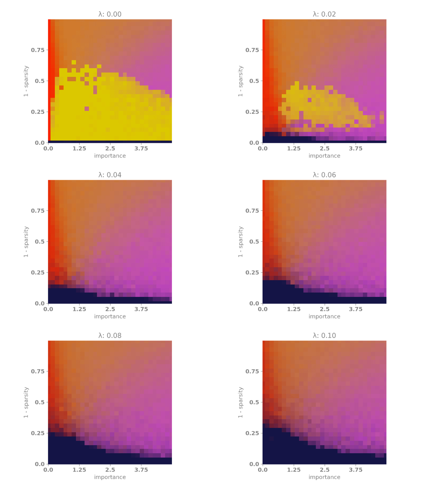
The following animation shows the results. A bright red color indicates that the network encoded only the first feature, which occurs when \(|W_1|\) is high and \(|W_2|\) is low. A bright purple color signifies that the network encoded only the second feature, happening when \(|W_1|\) is low and \(|W_2|\) is high. A bright yellow color means that the network encoded both features, which occurs when both \(|W_1|\) and \(|W_2|\) are high. Finally, when both \(|W_1|\) and \(|W_2|\) are low, the network did not encode any features, as it is more advantageous to minimize the regularization term. This last case is represented by a dark blue color.

On the x-axis, we have the relevance multiplier of the second feature with respect to the first one. When the relevance is low, the network prefers to encode the first feature, as indicated by the red vertical band on the left. When the relevance is high, the network favors encoding the second feature, as shown by the purple vertical band on the right. When the sparsity is high but \(\lambda\) is low, the network often opts for superimposing the features, represented by the yellow blob in the middle of the diagram. Finally, as \(\lambda\) and \(s\) increase, the network, in its effort to minimize the loss, simply chooses to set both weights to \(0\) and, therefore, does not encode any features. This is depicted by the dark blue band at the bottom of the diagram.
Despite my best efforts to obtain a clean phase diagram, the one I generated is quite noisy. Fortunately, we have a better way to visualize it, but it will require a bit of math. Specifically, we will find the expected value of the loss when \(W = [1, 0]\), \(W = [0, 1]\), \(W = [1, -1]\), and \(W=[0,0]\). \[\mathbb{E}_x[L(f(x);W)] = \iint_{[0,1]^2} p(x)L(f(x);W) \, dx_0 \, dx_1\]
Now, we will take into account the sparsity, specifically that \(p(x_i = 0) = s\). We have four cases:
- \(x_0 = 0, x_1 = 0\), which occurs with probability \(s^2\),
- \(x_0 = 0, x_1 \neq 0\), which occurs with probability \(s(1 - s)\),
- \(x_0 \neq 0, x_1 = 0\), which occurs with probability \((1 - s)s\),
- \(x_0 \neq 0, x_1 \neq 0\), which occurs with probability \((1 - s)^2\).
This results in the following integral: \[ \begin{aligned} \iint_{[0,1]^2} & s^2 \hspace{-.8cm} & L(f(x);W) dx_0 dx_1& + \\ \iint_{[0,1]^2} & s(1-s) \hspace{-.8cm} & L(f(x);W) dx_0 dx_1& + \\ \iint_{[0,1]^2} & (1-s)s \hspace{-.8cm} & L(f(x);W) dx_0 dx_1& + \\ \iint_{[0,1]^2} & (1-s)^2 \hspace{-.8cm} & L(f(x);W) dx_0 dx_1& \end{aligned} \] Now, we can also expand the loss: \[ \begin{aligned} & \iint_{[0,1]^2} s^2 \lambda \sum_{i=1}^n W_i^2 + \\ & \iint_{[0,1]^2} s(1-s) &\hspace{-1.7cm} \mathcal{L}(x;W) = \frac{1}{n} & \sum_{i=1}^n (f([0,x_2];W)_i - [0,x_2])^2 r_i & \hspace{-.8cm} + \lambda \sum_{i=1}^n W_i^2 & + \\ & \iint_{[0,1]^2} (1-s)s &\hspace{-1.7cm} \mathcal{L}(x;W) = \frac{1}{n} & \sum_{i=1}^n (f([x_1,0];W)_i - [x_1,0])^2 r_i & \hspace{-.8cm} + \lambda \sum_{i=1}^n W_i^2 & + \\ & \iint_{[0,1]^2} (1-s)^2 &\hspace{-1.7cm} \mathcal{L}(x;W) = \frac{1}{n} & \sum_{i=1}^n (f([x_1,x_2];W)_i - [x_1,x_2])^2 r_i & \hspace{-.8cm} + \lambda \sum_{i=1}^n W_i^2 & \end{aligned} \]
To you, this integral might look fine, but for me, it's beyond what I can tolerate. So, I will use a little trick and bring in SymPy, a Python library that can help us solve this integral. First, we need to let SymPy know which symbols we intend to use:
w1, w2, x1, x2, r1, r2 = sp.symbols('w1 w2 x1 x2 r1 r2')
lb, s = sp.symbols('lambda, s')
W = sp.Matrix([w1,w2])
x = sp.Matrix([x1,x2])
r = sp.Matrix([r1,r2])
Next, we will define a helper function that will return to us each term of the integral.
def get_expression_piece(x,W,r,z,sterm,lamb):
    x = z.multiply_elementwise(x).T
    f = (x @ W @ W.T).applyfunc(lambda v:sp.Max(v,0))
    return sterm * (((f - x).applyfunc(lambda x:x**2)).dot(r) + \
           lamb*(W[0]**2 + W[1]**2))
Finally, we will have only to put together the pieces of the integral and solve it.
expression = get_expression_piece(x,W,r,sp.Matrix([[1],[1]]),(1-s)**2,lb) + \
             get_expression_piece(x,W,r,sp.Matrix([[0],[1]]),s*(1-s) ,lb) + \
             get_expression_piece(x,W,r,sp.Matrix([[1],[0]]),(1-s)*s ,lb) + \
             get_expression_piece(x,W,r,sp.Matrix([[0],[0]]),s**2    ,lb)

print(sp.integrate(expression.subs({w1:0 , w2:0}),(x1, 0, 1),(x2, 0, 1)).simplify())
print(sp.integrate(expression.subs({w1:1 , w2:0}),(x1, 0, 1),(x2, 0, 1)).simplify())
print(sp.integrate(expression.subs({w1:0 , w2:1}),(x1, 0, 1),(x2, 0, 1)).simplify())
print(sp.integrate(expression.subs({w1:-1, w2:1}),(x1, 0, 1),(x2, 0, 1)).simplify())
This will return us with the following results:
- When we set \(W=[0,0]\), we have an expected loss of \( -s\frac{r_1}{3} + \frac{r_1}{3} - s\frac{r_2}{3} + \frac{r_2}{3}\).
- When we set \(W=[1,0]\), we have an expected loss of \( \lambda - s\frac{r_2}{3} + \frac{r_2}{3} \)
- When we set \(W=[0,1]\), we have an expected loss of \( \lambda - s\frac{r_1}{3} + \frac{r_1}{3} \)
- When \(W=[1,-1]\), we have \( 2\lambda + s^2\frac{r_1}{6} - s\frac{r_1}{3} + \frac{r_1}{6} + s^2\frac{r_2}{6} - s\frac{r_2}{3} + \frac{r2}{6} \)
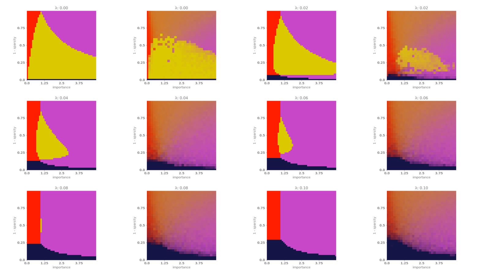
Now that we have these solutions, we can finally plot the theoretical phase diagram. The following animation displays the best of the four configurations for each value of \(\lambda\), \(s\), and \(r_2/r_1\). The color code remains the same as before: red indicates that the network encoded only the first feature, purple signifies that the network encoded only the second feature and yellow means that the network encoded both features. Finally, dark blue indicates that the network did not encode any features. We will also plot the empirical phase diagram for a nice side-by-side comparison.

As we can see, the theoretical phase diagram is much cleaner than the empirical one. Unfortunately, the theoretical diagram does not match the empirical one perfectly, but it is not too far off. Here, we can easily observe that as the regularization factor increases, the network tends to encode only one feature or none at all, avoiding superposition. This may not be desirable in some scenarios, so it is important to take this into account when designing a loss.